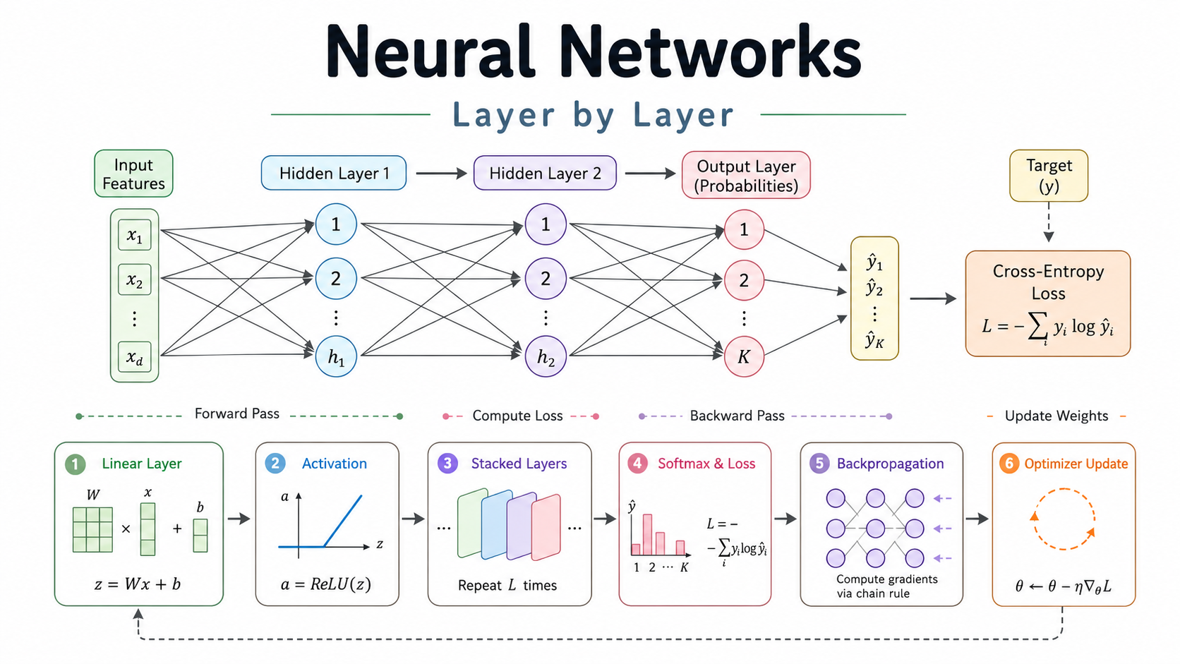
A neural network is a chain of functions. Each layer takes a tensor in, does one simple mathematical operation, and passes a tensor out. There’s no magic in it. It’s linear algebra, a nonlinearity, and calculus, repeated.
Here’s the chain in the order data actually flows through it: forward pass first, then how it learns. Every equation gets paired with its exact PyTorch equivalent, so you can see where the math actually lives in code.
- The Linear Layer
- Activation Function
- Stacking Layers
- Output Layer & Loss
- Backpropagation
- Optimizer Step
- The Training Loop
- Quick Reference
1. The Linear Layer
A single neuron computes one thing: a weighted sum of its inputs, plus a bias. Stack many neurons side by side and you get a “linear layer,” the workhorse of every network.
The math:
\[ z = Wx + b \]- \( x \in \mathbb{R}^n \): input vector (n features)
- \( W \in \mathbb{R}^{m \times n} \): weight matrix, one row per output neuron
- \( b \in \mathbb{R}^m \): bias vector, one shift per output neuron
- \( z \in \mathbb{R}^m \): pre-activation output (m features)
For a single output neuron this is just z = w·x + b = Σᵢ wᵢxᵢ + b, a dot product. Stacking m of these dot products into one matrix multiply is exactly what nn.Linear does.
Why a weighted sum? Every input feature might matter a different amount, and in a different direction, positive or negative. Weights
wencode how much and which way each feature should push the output. The biasblets the neuron shift its decision threshold independent of the inputs. Without it, every neuron would be forced to output 0 when x = 0, which is an arbitrary and usually wrong constraint.
PyTorch:
import torch
import torch.nn as nn

# n=4 input features, m=8 output features
layer = nn.Linear(in_features=4, out_features=8)

x = torch.randn(32, 4)     # batch of 32 samples, 4 features each
z = layer(x)                # z = x @ W.T + b

print(layer.weight.shape)   # torch.Size([8, 4])  -> W
print(layer.bias.shape)     # torch.Size([8])      -> b
print(z.shape)              # torch.Size([32, 8])
(32, 4) goes into Linear(4, 8) and comes out (32, 8).
2. Activation Function
Applied element-wise to z. It doesn’t mix features together. It just bends each number individually.
The math:
\[ a = \text{ReLU}(z) = \max(0, z) \]Two common alternatives you’ll see:
\[ \sigma(z) = \frac{1}{1+e^{-z}} \qquad \tanh(z) = \frac{e^{z}-e^{-z}}{e^{z}+e^{-z}} \]Why not just stack linear layers? Because a linear function of a linear function is still linear. Compose
W2(W1 x + b1) + b2and it collapses algebraically into a singleW'x + b'. No amount of stacking linear layers alone gets you more expressive power than one layer.The activation function is the only thing that breaks that collapse. It’s the only thing that lets a deep network represent curves, decision boundaries, anything non-straight-line.
ReLU is the default choice today because its gradient is either 0 or 1. That’s cheap, and it avoids the “vanishing gradient” problem that squashing functions like sigmoid and tanh cause in deep nets.
PyTorch:
relu = nn.ReLU()
a = relu(z)                 # same shape as z, negatives clipped to 0

# functional form, no module needed:
a = torch.relu(z)
(32, 8) goes into ReLU and comes out (32, 8). The shape never changes.
3. Stacking Layers
Repeat Linear then Activation a few times and you get a “deep” network. Each stage re-represents the data in a new feature space.
The math:
\[ \begin{aligned} a_1 &= \text{ReLU}(W_1 x + b_1) \\ a_2 &= \text{ReLU}(W_2 a_1 + b_2) \\ \hat{y} &= W_3 a_2 + b_3 \end{aligned} \]Here \( x \) is the raw input, \( a_1, a_2 \) are hidden representations (“hidden layers”), and \( \hat{y} \) is the raw model output before any final squashing.
Why more than one hidden layer? Each layer can only bend the space it’s given so far. One hidden layer already gives you a “universal approximator” in theory, but in practice it might need an enormous number of neurons to approximate a complex function.
Composing several moderate-width layers lets early layers learn simple, reusable features (edges, thresholds) and later layers combine those into more abstract ones (shapes, categories). That’s the same reason deep hierarchies are more parameter-efficient than one very wide layer.
PyTorch:
model = nn.Sequential(
    nn.Linear(4, 16),
    nn.ReLU(),
    nn.Linear(16, 16),
    nn.ReLU(),
    nn.Linear(16, 3),   # raw scores ("logits"), no activation yet
)

x = torch.randn(32, 4)
y_hat = model(x)
print(y_hat.shape)          # torch.Size([32, 3])
(32, 4) to (32, 16) to (32, 16) to (32, 3).
4. Output Layer & Loss
The last linear layer produces raw scores (“logits”). Softmax turns them into a probability distribution. The loss function turns that distribution into a single number to minimize.
The math:
\[ \text{softmax}(\hat{y})_i = \frac{e^{\hat{y}_i}}{\sum_j e^{\hat{y}_j}} \]\[ \mathcal{L} = -\log\big(p_{\text{true class}}\big) \]Here \( \hat{y} \) are the logits, unbounded raw scores, one per class. \( p = \text{softmax}(\hat{y}) \) are probabilities that sum to 1. And \( \mathcal{L} \) is the cross-entropy loss, which is 0 if the true class gets probability 1.
Why not just use accuracy directly? Accuracy is a step function. It doesn’t tell you how close you were, and its gradient is zero almost everywhere, so gradient descent has nothing to follow.
Softmax converts arbitrary logits into probabilities that are differentiable, always positive, and sum to 1. Cross-entropy then penalizes the model in proportion to
-log(p), which explodes as the predicted probability for the correct class goes to 0.That gives a smooth, strongly-sloped signal exactly where the model is most wrong, which is ideal for gradient-based learning.
PyTorch:
loss_fn = nn.CrossEntropyLoss()   # combines log-softmax + NLL loss internally

y_hat = model(x)                   # raw logits, shape (32, 3), do NOT softmax first
targets = torch.randint(0, 3, (32,))  # true class index per sample

loss = loss_fn(y_hat, targets)     # single scalar tensor
print(loss.item())
Note: nn.CrossEntropyLoss applies softmax internally for numerical stability. Feed it raw logits, never pre-softmaxed probabilities.
5. Backpropagation
To improve, every weight needs to know: if I nudge myself slightly, does the loss go up or down, and by how much? That’s a gradient, and backprop computes all of them in one backward sweep.
The math, the chain rule, applied through every layer:
\[ \frac{\partial \mathcal{L}}{\partial W_1} = \frac{\partial \mathcal{L}}{\partial \hat{y}} \cdot \frac{\partial \hat{y}}{\partial a_2} \cdot \frac{\partial a_2}{\partial z_2} \cdot \frac{\partial z_2}{\partial a_1} \cdot \frac{\partial a_1}{\partial z_1} \cdot \frac{\partial z_1}{\partial W_1} \]\( \partial \mathcal{L} / \partial W \) is how much a tiny change in W changes the loss. That’s the gradient. The chain rule just says the derivative of a composition is the product of each step’s derivative.
Why compute it backward, not forward? A network with L layers has a gradient expression that’s a product of L terms for every single weight. Computing that product separately for each of potentially millions of weights (forward-mode) is wasteful, because most of the terms are shared across weights.
Backprop computes the chain once from the loss backward to the inputs, reusing each intermediate derivative for every weight that depends on it. It’s just dynamic programming applied to the chain rule, and it’s the single reason training large networks is computationally feasible at all.
Chris Olah’s Calculus on Computational Graphs: Backpropagation is the canonical write-up of this argument. It makes the case visually with computational graphs and a path-counting argument for why reverse-mode wins whenever you have many inputs and one output, which is exactly a neural network’s shape.
PyTorch:
loss = loss_fn(model(x), targets)

loss.backward()   # walks the autograd graph backward,
                   # fills in .grad for every parameter

for name, p in model.named_parameters():
    print(name, p.grad.shape)   # gradient, same shape as the parameter itself
PyTorch built the computation graph automatically while you called model(x). That’s what “autograd” is. You never write the chain rule by hand.
Worked example, real numbers
The equations above are true for any depth, but they’re easiest to trust with an example small enough to check by hand: one linear neuron, no hidden layers, one sample, MSE loss.
Given: x = [1, 2], W = [0.5, -0.3], b = 0.1, target y = 1.0.
Forward pass, \( \hat{y} = W \cdot x + b \):
\[ \hat{y} = (0.5)(1) + (-0.3)(2) + 0.1 = 0.5 - 0.6 + 0.1 = 0.0 \]Loss, \( \mathcal{L} = (\hat{y} - y)^2 \):
\[ \mathcal{L} = (0.0 - 1.0)^2 = 1.0 \]How sensitive is the loss to the prediction?
\[ \frac{\partial \mathcal{L}}{\partial \hat{y}} = 2(\hat{y} - y) = 2(0.0 - 1.0) = -2.0 \]How sensitive is the prediction to each weight?
\[ \frac{\partial \hat{y}}{\partial w_i} = x_i \quad \Rightarrow \quad \frac{\partial \hat{y}}{\partial w_1} = 1,\ \ \frac{\partial \hat{y}}{\partial w_2} = 2 \]\( w_2 \) moves \( \hat{y} \) twice as fast as \( w_1 \), purely because \( x_2 = 2 \) is twice \( x_1 = 1 \). That’s leverage, not importance.
Chain them together. This is exactly what .grad holds:
So W.grad = [-2.0, -4.0] and b.grad = -2.0.
6. Optimizer Step
Backprop tells you the direction of steepest increase. The optimizer decides how far to step in the opposite direction.
The math:
\[ W \leftarrow W - \eta \, \frac{\partial \mathcal{L}}{\partial W} \]\( \eta \) (eta) is the learning rate, the step size. Adam extends this with per-parameter momentum and adaptive step sizes, but the core update, moving opposite the gradient, is unchanged.
Why move opposite the gradient? The gradient points in the direction of steepest increase of the loss. To make the loss smaller, you move the opposite way.
The learning rate η controls how big a step: too large and you overshoot the minimum or diverge, too small and training crawls. Plain SGD takes this literally every step.
Adam additionally tracks a running average of past gradients (momentum) and their magnitudes (adaptive scaling), which smooths out noisy gradients and lets different parameters take different effective step sizes. It usually converges faster in practice.
PyTorch:
optimizer = torch.optim.Adam(model.parameters(), lr=1e-3)

optimizer.zero_grad()   # clear .grad from the previous step
loss.backward()          # fill .grad again for this step
optimizer.step()         # W <- W - update, for every parameter
Worked example, continued
Picking up the gradients from section 5 (W.grad = [-2.0, -4.0], b.grad = -2.0), with learning rate η = 0.1:
\( w_2 \) moved by +0.4, double \( w_1 \)’s +0.2. Same leverage asymmetry from the “sensitive to each weight” step back in section 5, carried all the way through to the update size. This is the concrete reason input features get normalized before training.
Verify. Did the prediction move toward the target?
\[ \hat{y}_{\text{new}} = (0.7)(1) + (0.1)(2) + 0.3 = 1.2 \]It went from 0.0 to 1.2, target is 1.0. One step closed nearly the entire gap. It slightly overshot, since η = 0.1 was large relative to this toy example’s curvature.
import torch, torch.nn as nn

layer = nn.Linear(2, 1)
with torch.no_grad():
    layer.weight[:] = torch.tensor([[0.5, -0.3]])
    layer.bias[:] = torch.tensor([0.1])

x, y = torch.tensor([1.0, 2.0]), torch.tensor([1.0])
optimizer = torch.optim.SGD(layer.parameters(), lr=0.1)
loss_fn = nn.MSELoss()

optimizer.zero_grad()
y_hat = layer(x)
loss = loss_fn(y_hat, y)
loss.backward()
optimizer.step()

print(layer.weight, layer.bias)   # tensor([[0.7, 0.1]])  tensor([0.3])
7. The Training Loop
Training is nothing more than repeating five steps: forward pass, compute loss, zero old gradients, backward pass, optimizer step.
import torch
import torch.nn as nn

model = nn.Sequential(
    nn.Linear(4, 16),
    nn.ReLU(),
    nn.Linear(16, 16),
    nn.ReLU(),
    nn.Linear(16, 3),
)

loss_fn = nn.CrossEntropyLoss()
optimizer = torch.optim.Adam(model.parameters(), lr=1e-3)

# toy data: 200 samples, 4 features, 3 classes
X = torch.randn(200, 4)
y = torch.randint(0, 3, (200,))

for epoch in range(100):
    optimizer.zero_grad()          # (1) clear old gradients
    y_hat = model(X)                # (2) forward pass
    loss = loss_fn(y_hat, y)        # (3) compute loss
    loss.backward()                 # (4) backward pass (autograd)
    optimizer.step()                 # (5) update weights

    if epoch % 20 == 0:
        print(f"epoch {epoch:>3} | loss {loss.item():.4f}")
Why
zero_grad()first? PyTorch accumulates gradients into.gradby default, which is useful for gradient accumulation across mini-batches, rather than overwriting them. If you skipzero_grad(), each step’s gradient gets added on top of the last one, and your updates silently compound across epochs. It’s a very common bug.
8. Quick Reference
| Concept | Math | PyTorch |
|---|---|---|
| Weighted sum + bias | z = Wx + b | nn.Linear(in, out) |
| Nonlinearity | a = max(0, z) | nn.ReLU() |
| Stacked layers | f₃∘f₂∘f₁(x) | nn.Sequential(...) |
| Class probabilities | softmax(ŷ) | built into CrossEntropyLoss |
| Error signal | L = -log(p) | nn.CrossEntropyLoss() |
| Gradients via chain rule | ∂L/∂W | loss.backward() |
| Weight update | W ← W − η·∂L/∂W | optimizer.step() |
| Clear old gradients | reset ∂L/∂W to 0 | optimizer.zero_grad() |
Want to run this yourself instead of just reading it? There’s a companion Jupyter notebook, same order (linear, activation, stacking, loss, backprop, optimizer, training loop), but on a real make_moons dataset with a live decision-boundary plot that bends around the two crescents as it trains. The source, Python included, is on GitHub.